참조 :
한 권으로 끝내는 <판다스 노트>
https://e-koreatech.step.or.kr/
from IPython.display import Image
import numpy as np
import pandas as pd
import seaborn as sns
import warnings

warnings.filterwarnings("ignore")

df = sns.load_dataset('titanic')
df.head()df.describe()| survived | pclass | age | sibsp | parch | fare | |
| count | 891 | 891 | 714 | 891 | 891 | 891 |
| mean | 0.383838 | 2.308642 | 29.69912 | 0.523008 | 0.381594 | 32.20421 |
| std | 0.486592 | 0.836071 | 14.5265 | 1.102743 | 0.806057 | 49.69343 |
| min | 0 | 1 | 0.42 | 0 | 0 | 0 |
| 0.25 | 0 | 2 | 20.125 | 0 | 0 | 7.9104 |
| 0.5 | 0 | 3 | 28 | 0 | 0 | 14.4542 |
| 0.75 | 1 | 3 | 38 | 1 | 0 | 31 |
| max | 1 | 3 | 80 | 8 | 6 | 512.3292 |
문자열 컬럼에 대한 통계표도 확인할 수 있습니다.
- count: 데이터 개수
- unique: 고유 데이터의 값 개수
- top: 가장 많이 출현한 데이터 개수
- freq: 가장 많이 출현한 데이터의 빈도수
df.describe(include="object")| sex | embarked | who | embark_town | alive | |
| count | 891 | 889 | 891 | 889 | 891 |
| unique | 2 | 3 | 3 | 3 | 2 |
| top | male | S | man | Southampton | no |
| freq | 577 | 644 | 537 | 644 | 549 |
df.head()| survived | pclass | sex | age | sibsp | parch | fare | embarked | class | who | adult_male | deck | embark_town | alive | alone | |
| 0 | 0 | 3 | male | 22 | 1 | 0 | 7.25 | S | Third | man | TRUE | NaN | Southampton | no | FALSE |
| 1 | 1 | 1 | female | 38 | 1 | 0 | 71.2833 | C | First | woman | FALSE | C | Cherbourg | yes | FALSE |
| 2 | 1 | 3 | female | 26 | 0 | 0 | 7.925 | S | Third | woman | FALSE | NaN | Southampton | yes | TRUE |
| 3 | 1 | 1 | female | 35 | 1 | 0 | 53.1 | S | First | woman | FALSE | C | Southampton | yes | FALSE |
| 4 | 0 | 3 | male | 35 | 0 | 0 | 8.05 | S | Third | man | TRUE | NaN | Southampton | no | TRUE |
0. 통계함수 옵션 :
skipna =True
axis = 0
1. 데이터 개수 : count
df.count()df['age'].count()
2. 조건에 해당하는 데이터의 평균구하기
condition = (df['adult_male'] == True)
df.loc[condition, 'age'].mean()
df.loc[cond,'age'].mean(skipna=True)
3. 중간값 구하기 : 홀수 데이터셋은 가운데 2개 데이터의 평균값
pd.Series([1, 2, 3, 4, 5, 6]).median()
4. 합계 구하기
df.loc[:,['age','fare']].sum()
5. cumsum() - 누적합, cumprod() - 누적곱
df['age'].cumsum()
6. var() - 분산
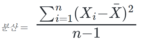
df['fare'].var()
7. 표준편차

df["fare"].std()
8. min() - 최소값, max() - 최대값
9. agg - aggregation: 통합 통계 적용 (복수의 통계 함수 적용)
df['age'].agg(['min', 'max', 'count', 'mean'])df[['age', 'fare']].agg(['min', 'max', 'count', 'mean'])
10. quantile() - 분위( 주어진 데이터를 동등한 크기로 분할하는 지점)
- 10%의 경우 0.1을, 80%의 경우 0.8을 대입하여 값을 구합니다.
# 10% quantile
df['age'].quantile(0.1)
11. unique() - 고유값, nunique() - 고유값 개수
df['who'].unique()
array(['man', 'woman', 'child'], dtype=object)
df['who'].nunique()
3
12. mode() - 최빈값( 가장 많이 출현한 데이터)
df['who'].mode()
0    man
dtype: object
13. corr() - 상관관계 ( 컬럼(column)별 상관관계)
- -1~1 사이의 범위를 가집니다.
- -1에 가까울 수록 반비례 관계, 1에 가까울수록 정비례 관계를 의미합니다.
from IPython.display import Image
import numpy as np
import pandas as pd
import seaborn as sns
import warnings

warnings.filterwarnings("ignore")
df.corr()
| survived | pclass | age | sibsp | parch | fare | adult_male | alone | |
| survived | 1 | -0.338481 | -0.077221 | -0.035322 | 0.081629 | 0.257307 | -0.55708 | -0.203367 |
| pclass | -0.338481 | 1 | -0.369226 | 0.083081 | 0.018443 | -0.5495 | 0.094035 | 0.135207 |
| age | -0.077221 | -0.369226 | 1 | -0.308247 | -0.189119 | 0.096067 | 0.280328 | 0.19827 |
| sibsp | -0.035322 | 0.083081 | -0.308247 | 1 | 0.414838 | 0.159651 | -0.253586 | -0.584471 |
| parch | 0.081629 | 0.018443 | -0.189119 | 0.414838 | 1 | 0.216225 | -0.349943 | -0.583398 |
| fare | 0.257307 | -0.5495 | 0.096067 | 0.159651 | 0.216225 | 1 | -0.182024 | -0.271832 |
| adult_male | -0.55708 | 0.094035 | 0.280328 | -0.253586 | -0.349943 | -0.182024 | 1 | 0.404744 |
| alone | -0.203367 | 0.135207 | 0.19827 | -0.584471 | -0.583398 | -0.271832 | 0.404744 | 1 |
특정 컬럼에 대한 상관관계
df.corr()['survived']
survived      1.000000
pclass       -0.338481
age          -0.077221
sibsp        -0.035322
parch         0.081629
fare          0.257307
adult_male   -0.557080
alone        -0.203367
Name: survived, dtype: float64
'pandas' 카테고리의 다른 글
| 데이터 전처리, 추가, 삭제, 변환 (0) | 2023.12.12 |
|---|---|
| 복사와 결측치 (0) | 2023.12.12 |
| 조회, 정렬, 조건필터 (0) | 2023.12.11 |
| Excel 파일 다루기 (0) | 2023.12.11 |
| pandas 기본 (0) | 2023.11.30 |


댓글